Implementing HPF in MATLAB

In this post, we implement a spatial-domain High Pass Filter (HPF) in MATLAB. A high pass filter suppresses low-frequency (smooth) regions of an image and enhances high-frequency content such as edges and sharp transitions. Unlike the Low Pass Filter which blurs an image, the HPF makes edges more visible by computing the Laplacian of the image at every pixel.

MATLAB Code

% High Pass Filter (HPF) in MATLAB
% Applies a 3x3 Laplacian high-pass kernel to a grayscale image.
% The kernel: [-1 -1 -1; -1 8 -1; -1 -1 -1]
% Computes: HPF(i,j) = 8*center - sum_of_8_neighbours

clc;        % Clear the command window
clear all;  % Clear all workspace variables

% --- Load image ---
% Place your image in the MATLAB working directory.
originalImage = imread('hills.jpg');      % Read the colour image
grayImage     = rgb2gray(originalImage);  % Convert to grayscale

imageSize = size(grayImage);  % [rows, cols]

% Initialise output as double to avoid uint8 overflow
hpfImage = double(grayImage);

% --- Apply Laplacian HPF kernel ---
% Skip the border pixels (row/col 1 and last row/col)
% to avoid out-of-bounds indexing.
for i = 2 : imageSize(1) - 1
    for j = 2 : imageSize(2) - 1
        % Laplacian: multiply centre by 8, subtract all 8 neighbours
        hpfImage(i, j) = ...
            -double(grayImage(i-1, j-1)) ...
            -double(grayImage(i-1, j  )) ...
            -double(grayImage(i-1, j+1)) ...
            -double(grayImage(i,   j-1)) ...
          +8*double(grayImage(i,   j  )) ...
            -double(grayImage(i,   j+1)) ...
            -double(grayImage(i+1, j-1)) ...
            -double(grayImage(i+1, j  )) ...
            -double(grayImage(i+1, j+1));
    end
end

% --- Display results ---
subplot(1, 2, 1);
imshow(grayImage);
title('Original Grayscale Image');

subplot(1, 2, 2);
imshow(hpfImage, []);
title('High Pass Filtered Image');

How the Code Works

1. Image loading — The colour image is read with imread() and converted to grayscale with rgb2gray() to get a 2D pixel matrix.
2. Laplacian kernel — The 3×3 Laplacian kernel used here is:
   [-1 -1 -1; -1 8 -1; -1 -1 -1]
   It subtracts the sum of all 8 neighbours from 8 times the centre pixel. In smooth regions all neighbours are similar so the result is near zero; at edges the centre differs from its neighbours and the result is large.
3. Border handling — The loops run from index 2 to rows-1 and 2 to cols-1, skipping the outermost border pixels which have no complete 3×3 neighbourhood. The border pixels keep their original values.
4. double() cast — Pixel arithmetic is performed in double precision to prevent the uint8 saturation that would occur if values went below 0 or above 255.
5. imshow(hpfImage, []) — Passing [] as the display range tells MATLAB to auto-scale the output to the min–max range, making the edge-enhanced result visible even when the absolute values are small.

Sample Output

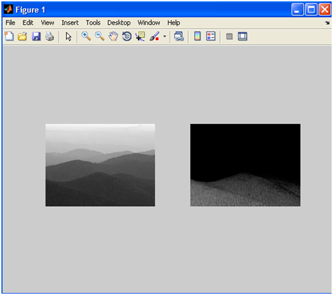
No text is printed to the command window. Running the script opens a figure showing the original grayscale image on the left and the high-pass filtered image on the right.

Output Explanation

1. Original Grayscale — The input image with full tonal range.
2. High Pass Filtered — Flat (uniform-colour) areas appear dark gray (near zero response). Object edges and textured regions appear bright because the pixel values differ significantly from their neighbours, producing a large Laplacian response. The image looks like an embossed or sketch-style rendering of the original.

See Also

• MATLAB Program to Implement LPF
• Implementing Edge Detection in MATLAB
• Program for Threshold in MATLAB
• Implementation of Histogram Processing in MATLAB

Conclusion

The spatial-domain high pass filter using the Laplacian kernel is a straightforward way to highlight edges and fine detail in an image. It is the spatial-domain counterpart to the frequency-domain HPF that attenuates low frequencies. Comparing this result with the output of the Low Pass Filter and the dedicated edge detectors provides a clear picture of how different filtering strategies affect image content.