
In this post, we implement a spatial-domain Low Pass Filter (LPF) in MATLAB using a 3×3 averaging kernel. A low pass filter smooths an image by replacing each pixel with the average of itself and its 8 neighbours. This reduces noise and high-frequency detail (sharp edges), producing a blurred version of the original. It is the spatial counterpart of frequency-domain low-pass filtering and is the basis of many image smoothing techniques.
MATLAB Code
% Low Pass Filter (LPF) in MATLAB
% Applies a 3x3 averaging kernel (box filter) to a grayscale image.
% Each output pixel is the mean of the 3x3 neighbourhood centred on it.

clc;        % Clear the command window
clear all;  % Clear all workspace variables

% --- Load image ---
% Place your image in the MATLAB working directory.
originalImage = imread('sample.jpg');      % Read the colour image
grayImage     = rgb2gray(originalImage);   % Convert to grayscale

imageSize = size(grayImage);  % [rows, cols]

% Initialise the output image (same size as input)
lpfImage = grayImage;

% --- Apply 3x3 averaging kernel ---
% Skip the border row/column (index 1 and last) to avoid out-of-bounds access.
for i = 2 : imageSize(1) - 1
    for j = 2 : imageSize(2) - 1
        % Sum the 3x3 neighbourhood and divide by 9 (average)
        lpfImage(i, j) = ( ...
            double(grayImage(i-1, j-1)) + double(grayImage(i-1, j)) + double(grayImage(i-1, j+1)) + ...
            double(grayImage(i,   j-1)) + double(grayImage(i,   j)) + double(grayImage(i,   j+1)) + ...
            double(grayImage(i+1, j-1)) + double(grayImage(i+1, j)) + double(grayImage(i+1, j+1))  ...
        ) / 9;
    end
end

% --- Display results ---
subplot(1, 2, 1);
imshow(grayImage);
title('Original Grayscale Image');

subplot(1, 2, 2);
imshow(lpfImage);
title('Low Pass Filtered (Blurred)');
How the Code Works
- Image loading — The colour image is read and converted to grayscale to give a 2D pixel matrix where each value is 0–255.
- Averaging kernel — The 3×3 box filter assigns equal weight (1/9) to every pixel in the 3×3 neighbourhood. The result is the arithmetic mean of those 9 pixels, which smooths abrupt intensity changes.
- Border handling — The nested loops run from row/column index 2 to
size - 1, deliberately skipping the outermost border. Border pixels retain their original values because they do not have a complete 3×3 neighbourhood. - double() cast — Each pixel is cast to
doublebefore arithmetic to prevent integer overflow during the summation. - subplot(1, 2, k) — Shows the original and filtered images side by side so the blurring effect is immediately visible.
Sample Output
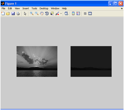
No text is printed to the command window. MATLAB opens a figure window showing the original grayscale image on the left and the blurred, low-pass filtered image on the right.
Output Explanation
- Original Grayscale — Full detail and sharpness, with clear edges between regions of different intensity.
- Low Pass Filtered — The image appears visibly blurred. Sharp edges are softened because the averaging operation mixes the high-intensity edge pixel with its lower-intensity neighbours, reducing the abrupt transition. Noise (random single-pixel variations) is also reduced because it is averaged out by the surrounding pixels.
See Also
- Implementing HPF in MATLAB
- Implementing Edge Detection in MATLAB
- Implementation of Histogram Processing in MATLAB
- Program for Threshold in MATLAB
Conclusion
The 3×3 averaging low pass filter is the simplest spatial smoothing technique in image processing. While a hand-coded nested loop clearly illustrates the concept, MATLAB’s built-in imfilter() or fspecial('average', [3 3]) provide a faster and more convenient way to apply the same operation in production code. Comparing the LPF result with the HPF result highlights the complementary nature of low-pass (smoothing) and high-pass (sharpening) filtering.
No Comments yet!