Plotting sin and cos Function in MATLAB

In this post, we plot the discrete-time sine and cosine functions in MATLAB using the stem() function. Sine and cosine are the most fundamental periodic signals in signal processing. Visualising them in the discrete-time domain helps build intuition for sampling, frequency analysis, and filter design.

MATLAB Code

% Plotting Discrete-Time sin and cos in MATLAB
% The user supplies n; the time axis runs from -n to +n.

clc;        % Clear the command window
clear all;  % Clear all workspace variables

% --- Sine plot ---
nSin = input('Enter n for sin plot : ');  % e.g. 5
tSin = -nSin:1:nSin;                     % Time axis: -n, ..., 0, ..., +n
ysin = sin(tSin);                        % Compute sin at each sample

subplot(1, 2, 1);
stem(tSin, ysin);
title('sin(n)');
xlabel('n');
ylabel('Amplitude');
ylim([-1.5, 1.5]);  % Fix y-axis for readability

% --- Cosine plot ---
nCos = input('Enter n for cos plot : ');  % e.g. 5
tCos = -nCos:1:nCos;                     % Time axis: -n, ..., 0, ..., +n
ycos = cos(tCos);                        % Compute cos at each sample

subplot(1, 2, 2);
stem(tCos, ycos);
title('cos(n)');
xlabel('n');
ylabel('Amplitude');
ylim([-1.5, 1.5]);  % Fix y-axis for readability

How the Code Works

1. Time axis — -n:1:n creates an integer sequence from -n to +n with step 1, giving 2n + 1 samples total (symmetric around zero).
2. Signal computation — MATLAB’s sin() and cos() functions operate element-wise on vectors, so sin(tSin) returns a vector of sin values at each integer sample.
3. stem() — Unlike plot(), which draws a continuous line, stem(t, y) draws vertical lines with dots to emphasise that the signal exists only at discrete integer values of n.
4. subplot(1, 2, k) — Places the sine and cosine plots side by side in one figure window (1 row, 2 columns).
5. ylim — Locks the y-axis to [-1.5, 1.5] so both subplots share the same scale, making the comparison accurate.

Sample Input / Output

Enter n for sin plot : 5
Enter n for cos plot : 5

ysin =
  Columns 1 through 9:
    0.9589    0.7568   -0.1411   -0.9093   -0.8415         0    0.8415    0.9093    0.1411
  Columns 10 through 11:
   -0.7568   -0.9589

ycos =
  Columns 1 through 9:
    0.2837   -0.6536   -0.9900   -0.4161    0.5403    1.0000    0.5403   -0.4161   -0.9900
  Columns 10 through 11:
   -0.6536    0.2837

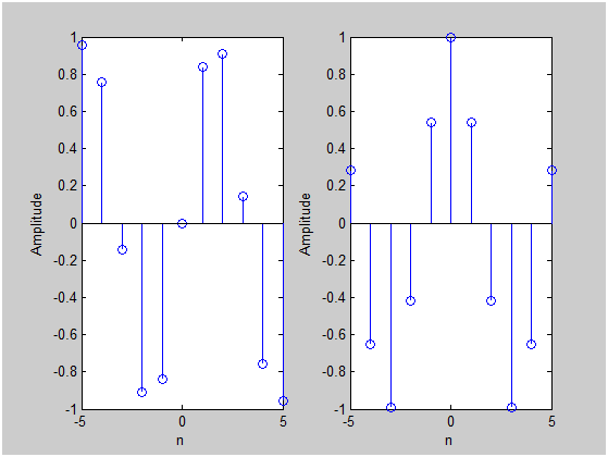
Output Explanation

1. For n = 5, the time axis is [-5, -4, -3, -2, -1, 0, 1, 2, 3, 4, 5] — 11 samples in total.
2. The sine values are non-zero at n = 0 (value 0) and oscillate between approximately −1 and +1. Note that sin(0) = 0 exactly, visible as the zero-height stem at the centre.
3. The cosine values show cos(0) = 1 at the centre, and the cosine starts at maximum, confirming the expected 90° phase lead over the sine.
4. Both subplots clearly show the oscillatory nature of sinusoidal signals even in the discrete domain.

See Also

• Plotting Unit Impulse, Unit Step, Unit Ramp and Exponential Function in MATLAB
• Plotting Linear and Circular Convolution with MATLAB
• Implementing DFT in MATLAB
• Implementing DCT and IDCT in MATLAB

Conclusion

This MATLAB program demonstrates how to generate and visualise discrete-time sine and cosine signals. The use of stem() is important here because it correctly conveys the discrete nature of the signals, unlike a continuous line plot. Sinusoidal signals are the basis of Fourier analysis; once you are comfortable plotting them, the next natural step is the Discrete Fourier Transform (DFT).