In this post, we implement the Discrete Fourier Transform (DFT) in MATLAB using the built-in fft() function and plot the resulting frequency-domain representation of a user-supplied sequence. The DFT converts a finite-length discrete-time signal from the time domain into the frequency domain, revealing which frequency components are present and at what amplitudes.

MATLAB Code

% Implementing DFT in MATLAB using fft()
% The user supplies a sequence and the DFT length.
% The magnitude spectrum is plotted using stem().

clc;        % Clear the command window
clear all;  % Clear all workspace variables

% --- Input ---
xSignal  = input('Enter the input sequence (e.g. [0.25 0.25 0.25 0]) : ');
nPoints  = input('Enter the DFT length N                              : ');

% --- Compute DFT ---
% fft(x, N) computes the N-point FFT (a fast algorithm for the DFT).
% If N > length(x), the sequence is zero-padded.
% If N < length(x), the sequence is truncated.
dftResult = fft(xSignal, nPoints);

% --- Compute magnitude spectrum ---
magnitude = abs(dftResult);   % |X(k)| for each frequency bin k

% --- Plot ---
figure;
subplot(1, 2, 1);
stem(real(dftResult));
title('DFT - Real Part');
xlabel('Frequency Bin (k)');
ylabel('Re{X(k)}');

subplot(1, 2, 2);
stem(imag(dftResult));
title('DFT - Imaginary Part');
xlabel('Frequency Bin (k)');
ylabel('Im{X(k)}');

% Display the magnitude spectrum in a separate figure
figure;
stem(magnitude);
title('DFT Magnitude Spectrum |X(k)|');
xlabel('Frequency Bin (k)');
ylabel('|X(k)|');

How the Code Works

1. User input — The user enters a row vector (the signal) and the DFT length N. If N equals the signal length, a standard DFT is computed. If N is larger, the signal is zero-padded, which increases frequency resolution in the plot.
2. fft(x, N) — MATLAB uses the Fast Fourier Transform (FFT) algorithm, which computes the DFT in O(N log N) time instead of O(N²). The result is a complex vector of length N.
3. abs(dftResult) — Computes the magnitude of each complex DFT coefficient: |X(k)| = √(Re² + Im²). The magnitude spectrum shows the energy at each frequency bin.
4. Real and imaginary plots — Two side-by-side subplots show the real and imaginary parts of the DFT separately, which helps understand the phase information.
5. Magnitude spectrum plot — A third standalone figure shows the magnitude, which is typically the most useful representation for analysing signal content.

Sample Input / Output

Enter the input sequence (e.g. [0.25 0.25 0.25 0]) : [0.25 0.25 0.25 0]
Enter the DFT length N                              : 4

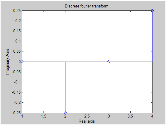
MATLAB opens figure windows showing the real part, imaginary part, and magnitude spectrum of the DFT.

Output Explanation

1. For x = [0.25, 0.25, 0.25, 0] and N = 4, the 4-point DFT gives: X(0) = 0.75, X(1) = 0.25 - 0.25j, X(2) = 0.25, X(3) = 0.25 + 0.25j.
2. DC component X(0) = 0.75 is the sum of all input values (the average scaled by N), representing the constant (zero-frequency) part of the signal.
3. The imaginary part is non-zero at bins 1 and 3, indicating that the signal has phase content at those frequencies.
4. The magnitude spectrum shows the largest value at bin 0 (DC), with smaller values at bins 1 and 3, confirming that the signal has most of its energy at low frequencies.

See Also

• Implementing DCT and IDCT in MATLAB
• Plotting Linear and Circular Convolution with MATLAB
• Plotting sin and cos Function in MATLAB
• Plotting Unit Impulse, Unit Step, Unit Ramp and Exponential Function in MATLAB

Conclusion

The DFT is the cornerstone of digital signal processing. This MATLAB program demonstrates how to compute it using the efficient FFT algorithm and how to interpret the resulting complex coefficients as a magnitude and phase spectrum. Building on this foundation, the next logical topics to explore are the DCT (used in image compression) and convolution in the frequency domain via the convolution theorem.