In this post, we implement Linear Convolution and Circular Convolution in MATLAB and plot both results side by side. Convolution is a fundamental operation in signal processing used to find the output of a Linear Time-Invariant (LTI) system when an input signal is applied to it.

Linear convolution computes the full convolution of two sequences, producing an output of length M + N - 1. Circular convolution (also called cyclic convolution) wraps around the result and is the basis of fast frequency-domain filtering using the DFT.

MATLAB Code

% Linear and Circular Convolution in MATLAB
% Reads two sequences from the user, computes both convolutions,
% displays the numerical results and plots all four signals.

clc;        % Clear the command window
clear all;  % Clear all workspace variables

% --- Input ---
x = input('Enter first sequence  : ');   % e.g. [1 1 2 2]
y = input('Enter second sequence : ');   % e.g. [1 2 3 4]

% --- Linear Convolution ---
% conv() returns a vector of length length(x)+length(y)-1
z = conv(x, y);
disp('Linear convolution result:');
disp(z);

% --- Circular Convolution ---
% cconv(x, y) uses the length of the longer sequence by default
c = cconv(x, y);
disp('Circular convolution result:');
disp(c);

% --- Plot all four signals ---
figure;

subplot(4, 1, 1);
stem(x);
title('First Input Sequence (x)');
xlabel('Sample Index');
ylabel('Amplitude');

subplot(4, 1, 2);
stem(y);
title('Second Input Sequence (y)');
xlabel('Sample Index');
ylabel('Amplitude');

subplot(4, 1, 3);
stem(z);
title('Linear Convolution  (z = x * y)');
xlabel('Sample Index');
ylabel('Amplitude');

subplot(4, 1, 4);
stem(c);
title('Circular Convolution  (c = x ⊛ y)');
xlabel('Sample Index');
ylabel('Amplitude');

How the Code Works

1. Input sequences — The user enters two row vectors. For example, x = [1 1 2 2] and y = [1 2 3 4].
2. Linear convolution (conv) — MATLAB’s built-in conv(x, y) slides one sequence over the other and sums the element-wise products at each shift. The output has length(x) + length(y) - 1 = 7 samples.
3. Circular convolution (cconv) — cconv(x, y) performs time-domain circular (cyclic) convolution. The result has the same length as the longer of the two input sequences.
4. Display — disp() prints the computed vectors to the command window so the user can verify the numbers before looking at the plot.
5. Subplots — subplot(4, 1, k) divides the figure window into four rows and one column, placing the k-th signal in the k-th row. stem() draws a discrete-time signal graph (vertical lines topped with dots).

Sample Input / Output

Enter first sequence  : [1 1 2 2]
Enter second sequence : [1 2 3 4]

Linear convolution result:
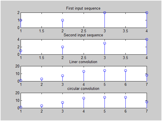
     1     3     7    13    14    14     8

Circular convolution result:
    1.0000    3.0000    7.0000   13.0000   14.0000   14.0000    8.0000

Output Explanation

For x = [1 1 2 2] and y = [1 2 3 4]:

1. Linear convolution produces 7 values: [1, 3, 7, 13, 14, 14, 8]. You can verify the first value: 1×1 = 1, the second: 1×2 + 1×1 = 3, and so on.
2. Circular convolution for this particular input produces the same numerical values because neither sequence wraps around (the circular length equals the linear output length here). In general, circular and linear convolution differ.
3. The four stem plots in the figure window show the input and output signals as discrete-time sequences, making it easy to compare shape and magnitude.

See Also

• Implementing DFT in MATLAB
• Implementing DCT and IDCT in MATLAB
• Plotting sin and cos Function in MATLAB
• Plotting Unit Impulse, Unit Step, Unit Ramp and Exponential Function in MATLAB

Conclusion

This MATLAB program demonstrates both linear and circular convolution of two discrete-time sequences. Linear convolution is used to compute the exact output of an LTI system, while circular convolution is closely tied to the DFT and is used in efficient frequency-domain filtering. Understanding the difference between the two is essential for any signal processing application.