In this post, we implement two basic image transformations in MATLAB: converting a colour image to grayscale and producing its digital negative. The digital negative inverts the intensity of every pixel — dark areas become light and vice versa — by applying the transformation s = 255 - r to each pixel value r. These are fundamental point processing operations in digital image processing.

MATLAB Code

% Digital Negative and Grayscale of an Image in MATLAB
% Demonstrates two point-processing transformations:
%   1. RGB -> Grayscale
%   2. Grayscale -> Digital Negative

clc;        % Clear the command window
clear all;  % Clear all workspace variables

% --- Load the image ---
% Place your image in the MATLAB working directory.
originalImage = imread('desert.jpg');    % Read a colour (RGB) image

% --- Convert to Grayscale ---
grayImage = rgb2gray(originalImage);     % Average the R, G, B channels

% --- Compute Digital Negative ---
% For an 8-bit image the maximum intensity is 255.
% Negative: negative(x,y) = 255 - gray(x,y)
negativeImage = 255 - grayImage;

% Optionally save the negative image to disk
imwrite(negativeImage, 'negative.jpg');

% --- Display all three images side by side ---
subplot(1, 3, 1);
imshow(originalImage);
title('Original Colour Image');

subplot(1, 3, 2);
imshow(grayImage);
title('Grayscale Image');

subplot(1, 3, 3);
imshow(negativeImage);
title('Digital Negative');

How the Code Works

1. imread() — Reads the image file from the current MATLAB working directory into a 3D matrix of size rows × cols × 3 (one layer per colour channel: R, G, B).
2. rgb2gray() — Converts the three-channel colour image into a single-channel grayscale image using the luminosity formula: Y = 0.299R + 0.587G + 0.114B. The result is a 2D matrix with values 0–255.
3. Digital Negative — The expression 255 - grayImage is applied element-wise to every pixel. A pixel with value 0 (black) becomes 255 (white), and a pixel with value 255 becomes 0. Mid-tones are symmetrically inverted.
4. imwrite() — Saves the negative image as a JPEG file in the working directory for later use.
5. subplot(1, 3, k) — Displays the three images (original, grayscale, negative) side by side in a single figure window using imshow().

Sample Output

Running the program with any colour JPEG opens a figure with three subplots. No numerical console output is generated; the result is entirely visual.

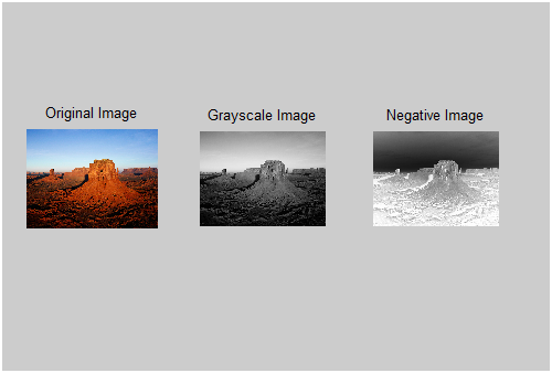
Output Explanation

1. Original Colour Image — The full-colour input image as loaded from disk.
2. Grayscale Image — All colour information is removed. Bright areas (high R/G/B values) appear light gray; dark areas appear dark gray.
3. Digital Negative — Every intensity is flipped. What was bright in the grayscale image is now dark, and vice versa. Sky appears dark, shadows appear light — similar to a photographic film negative.

See Also

• Gray-Level Slicing in MATLAB
• Implementation of Histogram Processing in MATLAB
• Program for Threshold in MATLAB
• Implementing Edge Detection in MATLAB

Conclusion

This program covers two of the most basic yet important operations in digital image processing: grayscale conversion and digital negative. Both are examples of point processing — each output pixel depends only on the corresponding input pixel, independent of its neighbours. These transformations are the foundation for more advanced techniques such as histogram equalisation, thresholding, and edge detection.