In this post, we use MATLAB to plot four fundamental discrete-time signals: the Unit Impulse, Unit Step, Unit Ramp, and Exponential Function. These signals are the building blocks of digital signal processing (DSP) and control systems theory. Understanding how to generate and visualize them in MATLAB is the first step towards analyzing more complex systems.

MATLAB Code

% Plotting Unit Impulse, Unit Step, Unit Ramp and Exponential Function
% All four signals are plotted in a 2x2 subplot grid.

clc;        % Clear the command window
clear all;  % Clear all workspace variables

% --- 1. Unit Impulse (delta function) ---
% Non-zero only at n=0; value = 1 at origin, 0 elsewhere
t = -2:1:2;                         % Time axis: -2, -1, 0, 1, 2
impulse = [zeros(1,2), 1, zeros(1,2)]; % 1 only at center (t=0)
subplot(2, 2, 1);
stem(t, impulse);
title('Unit Impulse');
xlabel('n');
ylabel('delta(n)');

% --- 2. Unit Step ---
% Value = 1 for all n >= 0
nStep = input('Enter length for unit step  : ');  % e.g. 5
tStep = 0:1:nStep - 1;              % Time axis: 0, 1, ..., nStep-1
stepSignal = ones(1, nStep);        % All ones
subplot(2, 2, 2);
stem(tStep, stepSignal);
title('Unit Step');
xlabel('n');
ylabel('u(n)');

% --- 3. Unit Ramp ---
% Value increases linearly: r(n) = n for n >= 0
nRamp = input('Enter length for unit ramp   : ');  % e.g. 4
tRamp = 0:1:nRamp - 1;             % Time axis: 0, 1, ..., nRamp-1
subplot(2, 2, 3);
stem(tRamp, tRamp);                 % y = n (ramp equals the index)
title('Unit Ramp');
xlabel('n');
ylabel('r(n) = n');

% --- 4. Exponential Function ---
% y(n) = exp(a*n); decaying when a0
nExp = input('Enter length for exponential : ');  % e.g. 5
tExp = 0:1:nExp - 1;               % Time axis
a   = input('Enter exponent value (a)     : ');  % e.g. -0.5 or 2
expSignal = exp(a * tExp);
subplot(2, 2, 4);
stem(tExp, expSignal);
title('Exponential Function');
xlabel('n');
ylabel('e^{an}');

How the Code Works

1. Unit Impulse — A fixed time vector t = [-2, -1, 0, 1, 2] is created. The signal vector is built with zeros flanking a single 1 at the centre (index 3, corresponding to t = 0). This correctly represents the Kronecker delta δ(n).
2. Unit Step — The user specifies the length nStep. ones(1, nStep) creates a row vector of all 1s, representing u(n) = 1 for n ≥ 0.
3. Unit Ramp — The user specifies the length nRamp. Because r(n) = n, the time vector tRamp is also the signal value itself, so stem(tRamp, tRamp) is used.
4. Exponential Function — The user provides the length nExp and the base a. MATLAB computes exp(a .* tExp) element-wise. A negative a gives a decaying exponential; a positive a gives a growing one.
5. subplot(2, 2, k) — Arranges the four plots in a 2-row, 2-column grid. The stem() function is used throughout to emphasise the discrete nature of these signals.

Sample Input / Output

Enter length for unit step  : 5
Enter length for unit ramp   : 4
Enter length for exponential : 5
Enter exponent value (a)     : 2

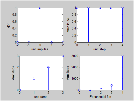
MATLAB opens a figure window showing all four subplots. The unit impulse is fixed; the remaining three signals reflect the user-supplied lengths and exponent.

Output Explanation

1. Unit Impulse — A single stem at n = 0 with amplitude 1. All other stems have amplitude 0, clearly showing the spiked nature of the delta function.
2. Unit Step (length 5) — Five stems at n = 0, 1, 2, 3, 4, each with amplitude 1. The flat top represents a constant signal that “switches on” at n = 0.
3. Unit Ramp (length 4) — Stems at n = 0, 1, 2, 3 with amplitudes 0, 1, 2, 3. The linearly increasing height gives the characteristic ramp shape.
4. Exponential (a = 2, length 5) — Stems at n = 0..4 with values approximately 1, 7.4, 54.6, 403.4, 2981. The rapidly growing height confirms the exponentially increasing nature when a > 0.

See Also

• Plotting sin and cos Function in MATLAB
• Plotting Linear and Circular Convolution with MATLAB
• Implementing DFT in MATLAB
• Implementing DCT and IDCT in MATLAB

Conclusion

This MATLAB program plots the four cornerstone discrete-time signals — unit impulse, unit step, unit ramp, and exponential. Mastery of these signals is essential before moving to topics such as convolution, DFT, and filter design, as virtually every DSP concept is built on top of these primitives.